Lab 2: Visualizing and Understanding the Sandbox Terrain Survey using ArcGIS
Visualizing and Understanding the Sandbox Terrain Survey using ArcGIS
Introduction
On Saturday, February 3rd,
a survey of a sandbox terrain was taken in the chilly February snow. The
sandbox was a 114 cm x 114 cm square located to the east of Phillips Hall on
the University of Wisconsin – Eau Claire campus. The survey group created a
terrain involving a ridge in the northern section of the sandbox with two hills
in the southern portion. A grid was set up containing 6 cm x 6 cm squares that
were used to perform a normal survey method. This lab utilizes ArcGIS software
to create a visualize of the sandbox surveyed that day.
Before analyzing this data, the excel
file needed to be normalized. Data normalization is simply the organization of
data so that it can be easily analyzed. According to Whatis.com, “Database
normalization is the process of organizing data into tables in such a way that
the results of using the database are always unambiguous and as intended”. This
lab uses a set of 400 data points that are entered into an excel sheet;
therefore before the use in ArcMap, the data was normalized.
A normal survey method was used in
this sandbox survey. This means that an even distribution of data points were
collected throughout the survey area. The interpolation of these data points in
lab will use the data points collected to calculate an elevation value for
every other point in the survey area. This then creates a digital elevation
model (DEM). The creation of various DEM’s using ArcMap allow the terrain to be
easily analyzed.
Methods
Interpolation
Methods:
- IDW: Inverse distance weighted interpolation uses a linearly weighted combination of a set of surrounding data points to determine the elevation of the unknown points. This method assumes that the further the data point the less influence it has on the unknown point. The advantages of IDW is that it is a simplistic model so not many parameters are needed to perform the interpolation. The simplicity of IDW is also its downfall, as this may cause error in some areas of the map. The use of IDW on this survey area, didn’t work very well. The interpolation caused many peaks and depressions to occur where the known data points were collected, which caused an odd looking DEM to be created (Figure 1).

Figure 1. Interpolation of sandbox terrain using IDW method.
- Natural Neighbors: This interpolation method uses a subset of data points to the unknown point and applies weights to the data points bases on the proportional distance from the point to create an interpolated new value. It is similar to IDW, but uses a more complicated interpolation technique. The advantages of natural neighbor interpolation is that the more advanced method allows one to set a limit on overshoots and undershoots to get more accurate results. A disadvantage is that is still a simplistic model that can vary with accuracy. Within this survey the natural neighbor technique still created some odd peaks and depressions like IDW, but they were less common (Figure 2).

Figure 2. Interpolation of the sandbox terrain using natural neighbor.
- Kriging: Kriging method also uses weights based on the distance from the unknown points, as well as, the overall spatial distribution of the arranged points. Kriging assumes that the distribution of the points reflects a spatial correlation that can be used to determine the surface variations. Kriging is best used in geology or soil science because it works well if there is a known spatially correlated distance within the data. One needs to be careful using kriging interpolation because it doesn’t pass through any of the known data points and may create values that are exaggerated. The kriging interpolation for this sandbox survey looks relatively good, but the method makes me weary that the results may be an exaggeration (Figure 3).

Figure 3. Interpolation of the sandbox terrain using kriging.
- Spline: Spline interpolation uses a mathematical function that minimizes overall surface curvature, which results in a smooth surface that has the same elevation values of the inputted data points. Advantages of the spline method is that it creates a smooth surface and its mathematical model is good for estimating points that are above or below the maximum and minimum known data points. The disadvantages of spline is that it doesn’t work well with data points that are close together and have extreme elevation differences, for example a cliff. For this survey, the spline method created a very good looking map and since this terrain didn’t have too dramatic of relief it represented the data well (Figure 4).

Figure 4. Interpolation of the sandbox terrain using spline.
- TIN: Triangular irregular networks is an interpolation method that creates a surface topography by triangulating a set of vertices or known data points. This method also has subsets, such as Delaunay triangulation. The TIN method is effective at storing large amounts of data and is able to describe a surface at different resolutions. Its major disadvantage is that it requires visual inspection to verify data. In this survey, TIN didn’t create a very realistic surface. The sandbox terrain was still very triangular and difficult to analyze (Figure 5).

Figure 5. Interpolation of the sandbox terrain using TIN.


ArcScene allows one to import
feature classes from ArcMap in order to see them in three dimensions. For this
survey, each interpolation feature class was able to be imported into ArcScene
individually and rotated to be analyzed in three dimensions. Once a helpful
image was produced using ArcScene and image was able to be exported in the
format of a JPEG. Using ArcScene an image from the north looking to the south
and an image from the south looking towards the north was exported for every
interpolation method to ensure consistency. The scale for every method varies
slightly as some needed a larger vertical exaggeration to show any major
topography. The vertical exaggeration is not labeled within the exported 3D
images, but the orientation of the are labeled within the caption below.
Results and Discussion
The IDW interpolation method
produced a DEM that was very data point based (see Figure 1). The known data
points were very distant peaks or depressions, which caused an non-appealing
DEM. Since, IDW keeps the exact values of the known data points those are known
to be accurate but the surrounding points seem to have dramatically different
elevations that don’t seem to be accurate by visual analyzes. This IDW
interpolation method doesn’t appear to use the known data points effectively in
the creation of an DEM.
The next method is natural neighbor
interpolation (see Figure 2). This method had some similar issues to the IDW
method. Natural neighbor also had areas of distant peaks and depressions that
were clearly from the known data points. This method was not as extreme as IDW
but the issue is still present. The use of the surveyed elevations is good, but
the use of these to interpolate the other elevation values doesn’t produce a
good looking map.
The next method is kriging (see
Figure 3). Kriging interpolation created the smoothest method so far but its
use of complicated mathematical functions is concerning for the accuracy of the
interpolation. Kriging is good in the use of known spatial correlated distances
between data points, but this survey didn’t include this. Therefore, the method
may be too complicated for these data points.
Spline interpolation was the next
method used (see Figure 4). Since spline uses a single surface and then adjusts
to fit the known data points, it created a smooth, good looking map. This method
took away all the exaggerated peaks and depressions that IDW and natural
neighbor contained so the real peaks and depressions had more of a focus. Since,
this terrain didn’t have dramatic relief this method worked best for visual analyzation.
The final results were from the TIN
method (see Figure 5). Since this method uses triangulation it created triangular
features throughout the survey area. This method makes visual analyze the most
difficult and appears the most inaccurate of the methods. Figure 6 is a
comparison of all of the above methods.
 |
| Figure 6. Comparison of all five interpolation methods used during this terrain analysis. |
Conclusion
This exercise included the creation
and surveying of a terrain within a 114 cm x 114 cm sandbox and then using
various interpolation methods to create digital elevation models of the
sandbox. This survey was similar to other field based surveys as one had to
determine the best survey method and the most accurate way to survey the
terrain. In a larger mapping project these aspects would also need to be
considered to successfully survey the designated area. Even though this
exercise was a good representation, it varied because of its small size and ability
to create the terrain. Since, the group decided on the terrain and since the
terrain was on such a small scale not much pre-investigation was needed on the
topography of the survey area. Before the survey of a larger survey area, more pre-work
will be needed before a survey strategy can be created. In most survey areas a
grid based survey is not realistic. Many survey areas would be much too large
for such an extensive grid.
For this exercise, various
interpolation methods were used to determine the elevation of the rest of the
survey area. Interpolation can also be very helpful tool for other data types
as well. For example, interpolation can be used to get water table levels for
surface water features or groundwater. It could also be used to assess the populations
of animal species in an area. Interpolation could be used in a wide variety of
situations. It is a analysis method that uses a known set of data points to
interpret the unknown values in between. Within this exercise, the
interpolation method of spline was the most fit for the set of data collected. It
created a smooth, good looking map that wasn’t over exaggerated and distorted.
References
What
is database normalization? - Definition from WhatIs.com. Retrieved February 08,
2018, from http://searchsqlserver.techtarget.com/definition/normalization
ArcGIS
Help. Retrieved February 08, 2018, from http://desktop.arcgis.com/en/arcmap/10.3/manage-data/tin/fundamentals-of-tin-surfaces.htm
Types
of Interpolation Methods. Retrieved February 12, 2018, from http://www.gisresources.com/types-interpolation-methods_3/

Comments
Post a Comment