Lab 10: Distance Azimuth Survey Method
Distance Azimuth Survey Method
Introduction
Technology
within the Geospatial field has exploded within the past few decades. This
technology can make surveying today very efficient and accurate, but sometimes
technology fails. Therefore, it is important to have an alternative method that
doesn’t need modern technology. This lab was used to learn the method of
distance azimuth. This method uses a GPS unit and a laser distance finder to
perform a survey.
This
labs goal was to collect some data on various tree species on Putnam Drive on
the University of Wisconsin- Eau Claire Campus (Figure 1). Putnam Drive is a
nature trail that runs east-west on the southern part of UW- Eau Claire’s lower
campus. Eau Claire was a lumber town, so many of the forests that are present
today have been replanted. Part of Putnam Drive was never harvested during this
time and therefore, Putnam Drive has some of the oldest trees in Eau Claire
along its path. This path is also home to wetlands and wildlife and is a very
integrated
 |
| Figure 1. Location map showing the region of the UW- Eau Claire campus that was surveyed during this lab. |
Methodology
There
was three different locations that various trees were assessed at. The data
that was collected on every tree was distance, azimuth, diameter, and tree
type. The location of where the surveyor was standing was also taken at each
location with a GPS device. This group had three members. One member was taking
distance and azimuth measurements with the laser distance finder. Another
member was moving from tree to tree to measure the diameter of the trunk and to
note the type of tree. Since, this group had no tree experts within it, the
trees were named based on the type of bark present. The final member of the
group was the recorder and wrote down all of the necessary information in the
field notebook.
The
first step in taking distance azimuth is to designated and mark a spot on the
ground where the individual with the laser distance finder will stand. Since,
the GPS location is taken from this spot, it is very important for this
individual to not move very far from this marked location. The next step is to
properly use the laser distance finder. To find the distance to the designated
tree, the finder can be pointed at the trunk at chest level and the laser
button can be hit (Figure 2). Make sure that the distance finder reads SD for
slope distance, this value is usually in meters. The next step is to adjust the
settings of the finder until it reads AZ for azimuth, the laser button can be
held again to determine the azimuth, this will be in degrees. This is all that
the individual with the laser distance azimuth needs to do for each tree.
 |
| Figure 2. A group member using the laser distance finder. |
The
individual that is going to each tree, simply uses the measuring tape to
measure the average diameter of the tree, which was in centimeters (Figure 3).
This person also needs to determine the type of tree. Since, no one was a tree
expert, this group chose to make three categories for type of tree. Smooth,
medium, and rough barked trees were the three categories used. The final member
of the group was recording this information down in an organized manner (Figure
4). The other members of the group were to read the measurements out loud for
the recorder to hear. Once, about four trees were recorded, the members of this
group decided to switch role, in order for everyone to get practice in. Once,
about nine trees were categorized within the first location this group decided
to move west to assess the trees at a different location. A new GPS location
was taken and the same parameters were followed to assess the trees at this new
location. After about four measurements, the group moved to a third and final
location. Only about three measurements were taken at this location.
 |
| Figure 3. Group member measuring the diameter of a tree of interest. |
 |
| Figure 4. Image of notes taken during the lab on distance, azimuth, tree type, and tree diameter. |
Once
the data was taken in the field, the next step is to type up this data into an
excel spreadsheet so it can be analyzed within ArcMap. A file geodatabase was
created for this project. The excel table was then imported into the
geodatabase. Next, the tool of Bearing Distance to Line command should be used
in ArcMap. This uses the azimuths and distances that were collected with the
laser distance finder to create a feature vertices. These feature vertices were
then made into points by using the Feature Vertices to Point Command. Now,
ArcMap shows all of the data points that were collected and the lines from the
standing location to the trees. The only issue left is that the created points
do not have all of the attributes that the table does. The final step is to do
a table join so the point data set will have all the correct information within
the attribute table.
Results
Once,
the tables were joined a base map was used and a map was created to show the
data collected (Figure 5). This map shows the distribution of trees collected
for this lab. Most of the trees collected were on the south side of Putnam
Drive, this was due to the wetland that is present to the north side of the
trail. It was a very wet day and our group didn’t navigate into this wetland;
thus, our data is skewed to the south portion of the trail. The first location
was the one located to the far east of the map. This group then moved west,
while collecting data on the trees.
 |
| Figure 5. A map of the data points taken on Putnam Drive. |
Conclusion
Geospatial
technology is a great thing to have and it can make the collection of data much
more efficient and accurate, but other methods need to be learned in case
technology can’t be used. The method of distance azimuth is an easy and
important skill to have as a back-up plan. All that was needed for this lab was
a laser distance finder, a GPS unit, and a measuring device to take data points
of tree diameter. This method was efficient and would work well if technology
was no longer in the picture.


Comments
Post a Comment